StatComp Project Example Solution: Numerical Statistics

Archaeology in the Baltic sea

Pairs of counts $(Y_{j,1},Y_{j,2})$ of left and right femurs from archaeological excavations are modelled as being conditionally independent realisations from $\textrm{Binom}(N_j,\phi)$ , where $N_j$ is the original number of people buried at each excavtion site, and $\phi$ is the probability of finding a buried femur. The prior distribution for each $N_j$ , $j=1,\dots,J$ , is $\textrm{Geom}(\xi)$ , where $\xi=1/(1+1000)$ (so that $\textrm{E}(N_j)=1000$ a priori), and for the detection probability, $\phi\sim\textrm{Beta}(\frac{1}{2},\frac{1}{2})$ . We denote $\boldsymbol{N}=\{N_1,\dots,N_J\}$ and $\boldsymbol{Y}=\{(Y_{1,1},Y_{1,2}),\dots,(Y_{J,1},Y_{J,2})\}$ .

Joint probability function

Taking the product of the prior density for $\phi$ , the prior probabilities for $N_j$ , and the conditional observation probabilities for $N_{j,i}$ and integrating over $\phi$ , we get the joint probability function for $(\boldsymbol{N},\boldsymbol{Y})$ $\begin{aligned} \textrm{P}(\boldsymbol{N},\boldsymbol{Y}) &= \int_0^1 p_\phi(\phi) \prod_{j=1}^J p(N_j) \prod_{i=1}^2 p(Y_{j,i}|N_j,\phi)\,\mathrm{d}\phi \\ &= \int_0^1 \frac{\phi^{a-1}(1-\phi)^{b-1}}{B(a,b)} \prod_{j=1}^J p(N_j) \prod_{i=1}^2 {N_j \choose Y_{j,i}} \phi^{Y_{j,i}}(1-\phi)^{N_j-Y_{j,i}} \,\mathrm{d}\phi \\ &= \int_0^1 \frac{\phi^{\widetilde{a}-1}(1-\phi)^{\widetilde{b}-1}}{B(a,b)} \,\mathrm{d}\phi\, \prod_{j=1}^J p(N_j) \prod_{i=1}^2 {N_j \choose Y_{j,i}} , \end{aligned}$ where $\widetilde{a} = a+\sum_{j=1}^J\sum_{i=1}^2 Y_{j,i}$ and $\widetilde{b} = b+\sum_{j=1}^J\sum_{i=1}^2 (N_j - Y_{j,i})$ . Then the integral can be renormalised to an integral of the distribution probability density function for a $\textrm{Beta}(\widetilde{a},\widetilde{b})$ distribution: $\begin{aligned} \textrm{P}(\boldsymbol{N},\boldsymbol{Y}) &= \frac{B(\widetilde{a},\widetilde{b})}{B(a,b)} \int_0^1 \frac{\phi^{\widetilde{a}-1}(1-\phi)^{\widetilde{b}-1}}{B(\widetilde{a},\widetilde{b})} \,\mathrm{d}\phi\, \prod_{j=1}^J p(N_j) \prod_{i=1}^2 {N_j \choose Y_{j,i}} \\ &= \frac{B(\widetilde{a},\widetilde{b})}{B(a,b)} \prod_{j=1}^J p(N_j) \prod_{i=1}^2 {N_j \choose Y_{j,i}} . \end{aligned}$

Credible intervals for $N_j$ and $\phi$

In order to obtain posterior credible intervals for the unknown quantities $\boldsymbol{N}=\{N_1,\dots,N_J\}$ , and $\phi$ , we implement an importance sampling method that sample each $N_j$ from a shifted Geometric distribution with smallest value equal to the smallest valid $N_j$ , given the observed counts, and expectation corresponding to $\phi=1/4$ . After sampling the $\boldsymbol{N}$ values, the corresponding importance weights $w_k$ , stored as Log_Weights equal to $\log(w_k)$ normalised by subtracting the larges $\log(w_k)$ value. Finally, $\phi$ values are sampled directly from the conditional posterior distribution $(\phi|\boldsymbol{N},\boldsymbol{Y})\sim\textrm{Beta}\left(\frac{1}{2}+\sum_{j,i} Y_{i,j},\frac{1}{2}+\sum_{j,i} (N_j-Y_{i,j})\right)$ . The implementation is in the arch_importance() function in my_code.R shown in the code appendix, and produces an importance sample of size $K$ . To achieve relatively reliable results, we use $K=100000$ , for each of $J=1$ , $2$ , $3$ , and $4$ , which takes ca 4 seconds on my computer.

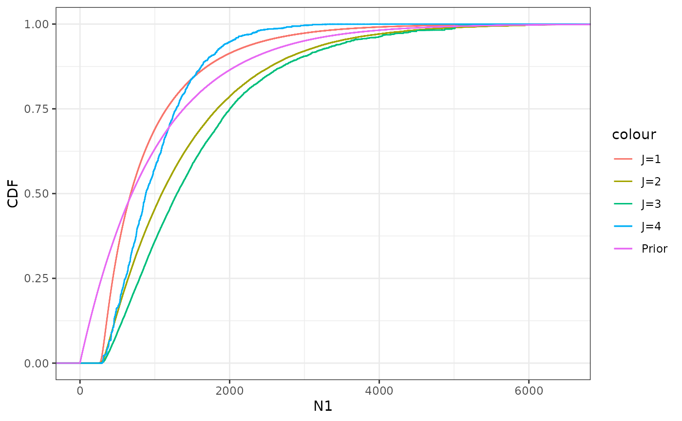
First, we use stat_ewcdf to plot the emprirical cumulative distribution functions for the importance weighted posterior samples of $N_1$ , for $J=1,\dots,4$ . We can see that the random variability increases for larger $J$ , indicating a lower efficiency of the importance sampler. Also included is the CDF for the prior distribution for $N_1$ . Except for the lower end of the distribution, it’s not immediately clear what effect the observations have on the distribution.

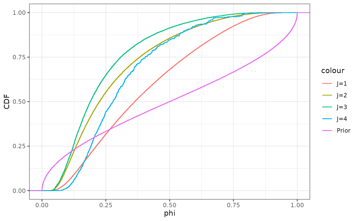
Next we do a corresponding plot for $\phi$ . In contrast to $N_1$ , here it’s more clear that the more observation pairs we get, the more concentrated the distribution for $\phi$ gets. Each new observation pair also influences in particular the lower end of the distribution, with the lower quantiles clearly increasing for $J=4$ even though the upper quantiles remain relatively stable for $J\geq 2$ .

Using wquantile to extract lower and upper $5\%$ quantiles we obtain approximate $90\%$ posterior credible intervals for $N_1$ and $\phi$ as shown in the following table.

J	Variable	Lower	Upper	Width
1	N1	313.0000000	2458.0000000	2145.0000000
2	N1	370.0000000	3454.0000000	3084.0000000
3	N1	421.0000000	3622.0000000	3201.0000000
4	N1	382.0000000	2023.0000000	1641.0000000
1	Phi	0.1000917	0.7881835	0.6880917
2	Phi	0.0710623	0.6668649	0.5958026
3	Phi	0.0680256	0.5849711	0.5169454
4	Phi	0.1223360	0.6525176	0.5301816

We can see that the credible intervals for $N_1$ are strongly linked to the information in the posterior distribution for $\phi$ . Interestingly, due to the lowering of the lower endpoint for $\phi$ for $J=2$ and $3$ , the width of the $N_1$ interval actually increases when we add the information from the second and third. This is stark contrast to our common intuition that would expect our uncertainty to decrease when we collect more data. The behaviour here is partly due to the random variability inherent in a small sample, but also due to the strong non-linearity of the estimation problem, where the products $\phi N_j$ are much easier to estimate than the individual $\phi$ and $N_j$ parameters. For $J=4$ , the interval width for $N_1$ finally decreases, as well as the width for the $\phi$ interval. Looking at the values of the observations, we can see that the $J=4$ case has much larger values than the other cases, which leads to it providing relatively more information about the $\phi$ parameter.

From a practical point of view, it’s clear that this estimation problem does not have an easy solution. Even with multiple excavations, and assuming that the model is appropriate and has the same value $\phi$ for $\phi$ for every excavation, we only gain a modest amount of additional information. On the positive side, if the model does a good job of approximating reality, then borrowing strength across multiple excavations does improve the estimates and uncertainty information for each excavation. For further improvements, one would likely need to more closely study the excavation precedures, to gain a better understanding of this data generating process, which might then lead to improved statistical methods and archaeologically relevant outcomes.

Extra

Effective sample size

Using the method for computing effective importance sample size from later in the course we can see that even with the more efficient method, the sampling is very inefficient for $J=4$ , indicating that an improved choice of importance distribution for $N_j$ could improve the precision and accuracy of the results:

J	EffSampleSize	RelEff
1	827101.3317	0.8271013
2	123325.1049	0.1233251
3	5652.0431	0.0056520
4	645.0274	0.0006450

Here, EffSampleSize is the approximate effective sample size $(\sum_k w_k)^2/\sum w_k^2$ , and RelEff is the relative efficiency, defined as the ratio between EffSampleSize and $K=100000$ .

Profile likelihood method for frequentist confidence interval for $\textrm{Binom}(n,p)$

## [1] 274

(actually range(y) depends on n may mean l0 not justified for this example)

Code appendix

Function definitions

# Finn Lindgren (s0000000, finnlindgren)



# Joint log-probability
#
# Usage:
#   log_prob_NY(N, Y, xi, a, b)
#
# Calculates the joint probability for N and Y, when
#   N_j ~ Geom(xi)
#   phi ~ Beta(a, b)
#   Y_{ji} ~ Binom(N_j, phi)
#   For j = 1,...,J
#
# Inputs:
#   N: vector of length J
#   Y: data.frame or matrix of dimension Jx2
#   xi: The probability parameter for the N_j priors
#   a, b: the parameters for the phi-prior
#
# Output:
#   The log of the joint probability for N and Y
#   For impossible N,Y combinations, returns -Inf

log_prob_NY <- function(N, Y, xi, a, b) {
  # Convert Y to a matrix to allow more vectorised calculations:
  Y <- as.matrix(Y)
  if (any(N < Y) || any(Y < 0)) {
    return(-Inf)
  }
  atilde <- a + sum(Y)
  btilde <- b + 2 * sum(N) - sum(Y) # Note: b + sum(N - Y) would be more general
  lbeta(atilde, btilde) - lbeta(a, b) +
    sum(dgeom(N, xi, log = TRUE)) +
    sum(lchoose(N, Y))
}

# Importance sampling for N,phi conditionally on Y
#
# Usage:
#   arch_importance(K,Y,xi,a,b)
#
# Inputs:
#   Y,xi,a,b have the same meaning and syntax as for log_prob_NY(N,Y,xi,a,b)
#   The argument K defines the number of samples to generate.
#
# Output:
#  A data frame with K rows and J+1 columns, named N1, N2, etc,
#  for each j=1,…,J, containing samples from an importance sampling
#  distribution for Nj,
#  a column Phi with sampled phi-values,
#  and a final column called Log_Weights, containing re-normalised
#  log-importance-weights, constructed by shifting log(w[k]) by subtracting the
#  largest log(w[k]) value, as in lab 4.

arch_importance <- function(K, Y, xi, a, b) {
  Y <- as.matrix(Y)
  J <- nrow(Y)
  N_sample <- matrix(rep(pmax(Y[, 1], Y[, 2]), each = K), K, J)
  xi_sample <- 1 / (1 + 4 * N_sample)

  N <- matrix(rgeom(K * J, prob = xi_sample), K, J) + N_sample
  colnames(N) <- paste0("N", seq_len(J))

  Log_Weights <- vapply(
    seq_len(K),
    function(k) log_prob_NY(N[k, , drop = TRUE], Y, xi, a, b),
    0.0) -
    rowSums(dgeom(N - N_sample, prob = xi_sample, log = TRUE))

  phi <- rbeta(K, a + sum(Y), b + 2 * rowSums(N) - sum(Y))

  cbind(as.data.frame(N),
        Phi = phi,
        Log_Weights = Log_Weights - max(Log_Weights))
}

Analysis code

Confidence intervals

Poisson parameter interval simulations:

Summarise the coverage probabilities and interval widths:

Plot the CDFs for the CI width distributions:

Archaeology

Compute credible intervals for $N_j$ for different amounts of data, $J$ :

xi <- 1 / 1001
a <- 0.5
b <- 0.5

K <- 1000000
NW1 <- arch_importance(K, arch_data(1), xi, a, b)
NW2 <- arch_importance(K, arch_data(2), xi, a, b)
NW3 <- arch_importance(K, arch_data(3), xi, a, b)
NW4 <- arch_importance(K, arch_data(4), xi, a, b)

For completeness, we compute all the credible intervals for $N_j$ , $1\leq J$ , for each $J=1,\dots,4$ , but the analysis focuses on $N_1$ and $\phi$ :

CI <- rbind(
  NW1 %>%
    reframe(
      J = 1,
      End = c("Lower", "Upper"),
      N1 = wquantile(N1,
        probs = c(0.05, 0.95), na.rm = TRUE,
        type = 1, weights = exp(Log_Weights)
      ),
      N2 = NA,
      N3 = NA,
      N4 = NA,
      Phi = wquantile(Phi,
        probs = c(0.05, 0.95), na.rm = TRUE,
        type = 7, weights = exp(Log_Weights)
      )
    ),
  NW2 %>%
    reframe(
      J = 2,
      End = c("Lower", "Upper"),
      N1 = wquantile(N1,
        probs = c(0.05, 0.95), na.rm = TRUE,
        type = 1, weights = exp(Log_Weights)
      ),
      N2 = wquantile(N2,
        probs = c(0.05, 0.95), na.rm = TRUE,
        type = 1, weights = exp(Log_Weights)
      ),
      N3 = NA,
      N4 = NA,
      Phi = wquantile(Phi,
        probs = c(0.05, 0.95), na.rm = TRUE,
        type = 7, weights = exp(Log_Weights)
      )
    ),
  NW3 %>%
    reframe(
      J = 3,
      End = c("Lower", "Upper"),
      N1 = wquantile(N1,
        probs = c(0.05, 0.95), na.rm = TRUE,
        type = 1, weights = exp(Log_Weights)
      ),
      N2 = wquantile(N2,
        probs = c(0.05, 0.95), na.rm = TRUE,
        type = 1, weights = exp(Log_Weights)
      ),
      N3 = wquantile(N3,
        probs = c(0.05, 0.95), na.rm = TRUE,
        type = 1, weights = exp(Log_Weights)
      ),
      N4 = NA,
      Phi = wquantile(Phi,
        probs = c(0.05, 0.95), na.rm = TRUE,
        type = 7, weights = exp(Log_Weights)
      )
    ),
  NW4 %>%
    reframe(
      J = 4,
      End = c("Lower", "Upper"),
      N1 = wquantile(N1,
        probs = c(0.05, 0.95), na.rm = TRUE,
        type = 1, weights = exp(Log_Weights)
      ),
      N2 = wquantile(N2,
        probs = c(0.05, 0.95), na.rm = TRUE,
        type = 1, weights = exp(Log_Weights)
      ),
      N3 = wquantile(N3,
        probs = c(0.05, 0.95), na.rm = TRUE,
        type = 1, weights = exp(Log_Weights)
      ),
      N4 = wquantile(N4,
        probs = c(0.05, 0.95), na.rm = TRUE,
        type = 1, weights = exp(Log_Weights)
      ),
      Phi = wquantile(Phi,
        probs = c(0.05, 0.95), na.rm = TRUE,
        type = 7, weights = exp(Log_Weights)
      )
    )
)

Restructure the interval data.frame to focus on $N_1$ and $\phi$ only:

CI_ <- CI %>%
  pivot_longer(
    cols = c(N1, N2, N3, N4, Phi),
    names_to = "Variable",
    values_to = "value"
  ) %>%
  pivot_wider(
    names_from = End,
    values_from = value
  ) %>%
  filter(!is.na(Lower)) %>%
  mutate(Width = Upper - Lower)
knitr::kable(CI_ %>% filter(Variable %in% c("N1", "Phi")) %>%
  arrange(Variable, J))

Finn Lindgren (s0000000, finnlindgren)