Tutorial 04: Uncertainty and integration (full solution)

Finn Lindgren

This document uses a code_folding: hide option to handle showing/hiding code when building locally. Download and build the source file from https://github.com/finnlindgren/StatCompLab/blob/main/vignettes/articles/T4sol.Rmd to see how that feature works.

Three alternatives for Poisson parameter confidence intervals

For case 3, the negated log-likelihood is $$\widetilde{l}(\theta) = n e^\theta - \theta \sum_{i=1}^n y_i + \text{constant}$$ with 1st order derivative $$\frac{\partial}{\partial\theta}\widetilde{l}(\theta) = n e^\theta - \sum_{i=1}^n y_i$$ which shows that $\widehat{\theta}_\text{ML}=\log(\overline{y})$, and 2nd order derivative $$\frac{\partial^2}{\partial\theta^2}\widetilde{l}(\theta) = n e^\theta$$ which is equal to $n\lambda$ for all $y_i$ values, so the inverse of the expected Hessian is $1/(n\lambda)$.

Interval construction

CI1 <- function(y, alpha = 0.05) {
  n <- length(y)
  lambda_hat <- mean(y)
  theta_interval <-
    lambda_hat - sqrt(lambda_hat / n) * qnorm(c(1 - alpha / 2, alpha / 2))
  pmax(theta_interval, 0)
}
CI2 <- function(y, alpha = 0.05) {
  n <- length(y)
  theta_hat <- sqrt(mean(y))
  theta_interval <-
    theta_hat - 1 / sqrt(4 * n) * qnorm(c(1 - alpha / 2, alpha / 2))
  pmax(theta_interval, 0)^2
}
CI3 <- function(y, alpha = 0.05) {
  n <- length(y)
  theta_hat <- log(mean(y))
  theta_interval <-
    theta_hat - 1 / sqrt(exp(theta_hat) * n) * qnorm(c(1 - alpha / 2, alpha / 2))
  exp(theta_interval)
}

We can test the interval construction methods with the following code.

y <- rpois(n = 5, lambda = 2)
print(y)
CI <- rbind(
  "Method 1" = CI1(y),
  "Method 2" = CI2(y),
  "Method 3" = CI3(y)
)
colnames(CI) <- c("Lower", "Upper")

	Lower	Upper
Method 1	0.7604099	3.239590
Method 2	0.9524829	3.431663
Method 3	1.0761094	3.717094

The methods will not always produce valid intervals.

• When $\overline{y}=0$, the first method produces a single point as “interval”.
• The third method fails if $\overline{y}=0$, due to log of zero.

This can happen when $n$ or $\lambda$ are close to zero.

Bayesian credible intervals

n <- 5
lambda <- 10
y <- rpois(n, lambda)
y # Actual values will depend on if set.seed() was used at the beginning of the document

## [1] 11  7 11  8  8

From probability theory, we know that $p(\theta)=p(\lambda) \frac{d\lambda(\theta)}{d\theta}$, so that $$p(\theta) = a \exp(-a\lambda) \exp(\theta) = a \exp\left( \theta-ae^\theta \right)$$

Importance sampling

First, we sample from the Gaussian approximation to the posterior distribution.

a <- 1/5
m <- 20000
x <- rnorm(m, mean = log(1+sum(y)) - log(a + n), sd = 1 / sqrt(1 + sum(y)))

To avoid numerical problems, we calculate the log of the unnormalised weights, and then shift the results to get a numerically sensible scale when we exponentiate.

log_weights <- (x * (1 + sum(y)) - (a + n) * exp(x)) -
 dnorm(x, mean = log(1 + sum(y)) - log(a + n), sd = 1 / sqrt(1 + sum(y)), log = TRUE)
weights <- exp(log_weights - max(log_weights))

The credible interval for $\theta$ can now be extracted from quantiles of the weighted sample, and the $\lambda$-interval is obtained by the transformation $\lambda=\exp(\theta)$:

theta_interval <- wquantile(x, probs = c(0.025, 0.975), weights = weights)
theta_interval

## [1] 1.873696 2.448506

lambda_interval <- exp(theta_interval)
lambda_interval

## [1]  6.512323 11.571043

The code for the above steps was the following:

a <- 1/5
m <- 20000
x <- rnorm(m, mean = log(1+sum(y)) - log(a + n), sd = 1 / sqrt(1 + sum(y)))

log_weights <- (x * (1 + sum(y)) - (a + n) * exp(x)) -
 dnorm(x, mean = log(1 + sum(y)) - log(a + n), sd = 1 / sqrt(1 + sum(y)), log = TRUE)
weights <- exp(log_weights - max(log_weights))

theta_interval <- wquantile(x, probs = c(0.025, 0.975), weights = weights)
theta_interval
lambda_interval <- exp(theta_interval)
lambda_interval

Cumulative distribution function comparison

The figure below shows the empirical distributions of the unweighted and weighted samples $\{x_k\}$ (with weights $\{w_k\}$), together with the theoretical posterior empirical distribution function. The weighted, importance sampling, version is virtually indistinguishable from the true posterior distribution. The unweighted sample is very close to the true posterior distribution; for this model, the Gaussian approximation of the posterior distribution of $\log(\lambda)$ is an excellent approximation even before we add the importance sampling step.

# Plotting updated to include a plot of the importance weights
p1 <-
  ggplot(data.frame(lambda = exp(x), weights = weights)) +
  ylab("CDF") +
  geom_function(fun = pgamma, args = list(shape = 1 + sum(y), rate = a + n),
                mapping = aes(col = "Theory")) +
  stat_ewcdf(aes(lambda, weights = weights, col = "Importance")) +
  stat_ecdf(aes(lambda, col = "Unweighted")) +
  scale_x_log10(limits = c(3, 20)) +
  labs(colour = "Type")

p2 <- ggplot(data.frame(lambda = exp(x), weights = weights),
             mapping = aes(lambda, weights / mean(weights))) +
  ylab("Importance weights") +
  geom_point() +
  geom_line() +
  geom_hline(yintercept = 1) +
  scale_y_log10() +
  scale_x_log10(limits = c(3, 20))

# The patchwork library provides a versatile framework
# for combining multiple ggplot figures into one.
library(patchwork)
(p1 / p2)

## Warning in geom_function(fun = pgamma, args = list(shape = 1 + sum(y), rate = a + : All aesthetics have length 1, but the data has 20000 rows.
## ℹ Please consider using `annotate()` or provide this layer with data containing
##   a single row.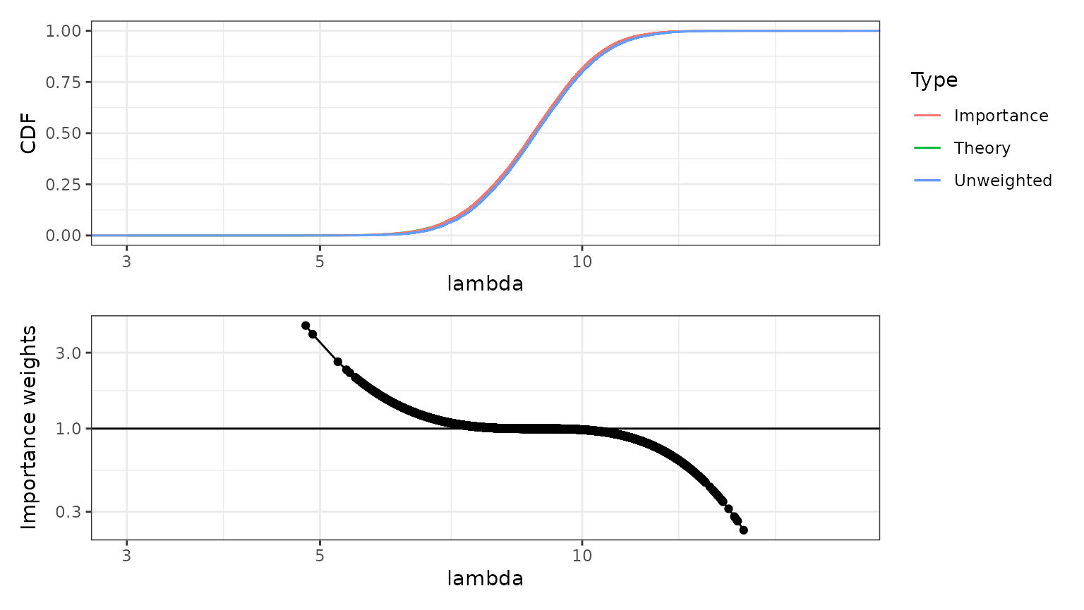

In the lower figure, the importance weights have be normalised by their average, so that values above 1 mean that the corresponding sample values should occur more often in the true, target, distribution than they do in the raw samples, and values below 1 mean that those sample values should occur less frequently in the target distribution. The scaled weights are shown on a logarithmic scale.